Introduction to Time and Frequency Domain

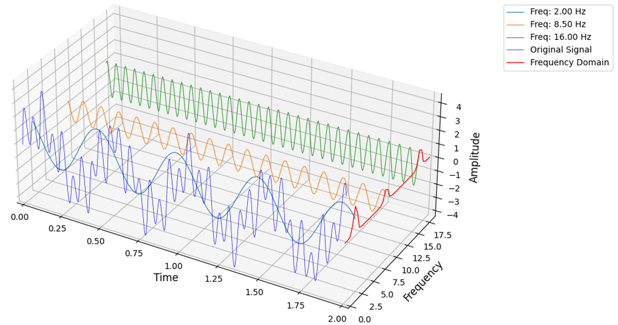
Understanding the time and frequency domains is fundamental in signal processing. Signals can be analysed in both domains to extract different types of information. While the time domain represents how a specific quantity changes over time, the frequency domain represents how much of the signal’s quantities lie within each given frequency band over a range of frequencies.

Time Domain

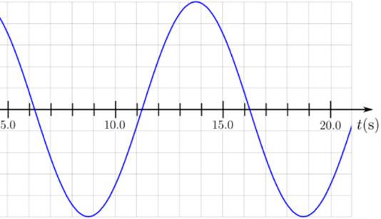
In the time domain, we observe the amplitude of some quantity of the signal as it changes over time. This is useful for understanding the temporal characteristics of the signal, such as duration, interval between events, any transient events, as well as absolute quantities like the maximum or minimum amplitudes observed during the event.

In mechanics, the maximum and minimum values present in a structure, such as strength, strain, acceleration, and deformation, play a crucial role in determining whether a structure is considered compliant. In the time domain, several actions occur simultaneously, and they can interfere constructively or destructively, leading to significant peaks and troughs in the response, which makes it straightforward to identify these maximum and minimum values. Nevertheless, there are statistical methods that can be used to calculate these peak values for the frequency domain.

Frequency Domain

In the frequency domain, we decompose the signal into its constituent frequencies. Most of the time, this is achieved through mathematical transformations of the time domain signal using the Fourier Transform. The frequency domain representation of a signal shows how much of the signal’s quantity is distributed across different frequencies. This helps in understanding the spectral content of the signal, identifying features or the absence of features, such as harmonic components, which aid in describing and characterising the signal.

In mechanics, the frequency domain is often used to identify natural frequencies of structures, damping characteristics, frequency content of the forcing input, noise in the system, amplification factors, and transfer functions. Additionally, the frequency domain can be easily modified by increasing or reducing the frequency content at certain frequencies. This process is known as signal filtering when reducing frequencies, and signal boosting or synthesis when increasing frequencies. These modifications can then be converted back to the time domain, resulting in a modified version of the original time signal.

Furthermore, certain operations are much simpler to perform in the frequency domain. For example, time fluctuating force on a structure in the time domain would need to be solved either numerically by stepwise, time-discretised calculation of high-order differential equations or by using the elaborate mathematical convolution method, which involves integrating the product of the input signal and the system’s impulse response over time to determine the overall response of the structure. In the frequency domain, however, they can be combined by simple multiplication of the forcing function in the frequency domain and the transfer function of the structure for that force.

Digital Signals

Real-world physical quantities are continuous and vary smoothly over time. In the case of dynamical systems, we usually look at deformations, velocities, accelerations, strains, or strain rates. These smooth variations over time can be mathematically described or approximated by continuous functions such as sinusoids, polynomials, or derivatives of Gaussian functions.

For example:

Sinusoids are defined as \(A \sin(2\pi f t + \phi)\), where \(A\) is the amplitude, \(f\) is the frequency, and \(\phi\) is the phase.

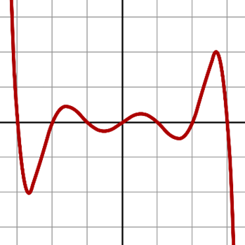
Polynomials are defined as \(a_0 + a_1 t + a_2 t^2 + a_3 t^3\), where \(a_n\) are constants.

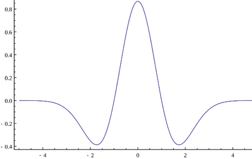
The Ricker wavelet is defined as \((1 - 2\pi^2 f_0^2 t^2) \cdot e^{-\pi^2 f_0^2 t^2}\), where \(f_0\) is the central frequency.

Using theories developed from dynamics on mechanical systems, we can perform operations on these continuous functions to derive other properties, which will also be represented in a continuous way. However, this limits us to operations on functions that we already know how to describe continuously. If we want to investigate a signal that we are not sure of or if we want to corroborate mathematical predictions with real-world examples, we need to take measurements of the quantity of interest.

Many measurement devices, such as accelerometers, seismographs, strain gauges, and temperature sensors, are analog and capture the smooth variation of signals, meaning they are continuous. Often, this provides enough information if you are just interested in simple concepts like peak values, timing of a peak, periodicity or the general shape of the signal. However, we are often interested in other properties of the signal that involve mathematical operations. Since it is often impossible to discern the mathematical expression or combination of expressions that form the recorded analog signal, it is in our best interest to transform it into a digital signal. This is because, computers are capable (and often faster) at performing similar calculations for discrete information as they are for continuous cases. This allows us to leverage the computational advantages of computers to perform the needed operations.

From Continuous to Discrete Signals

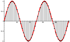
To achieve this transformation, continuous signals, which are analog signals that vary smoothly over time, need to be converted into discrete signals, which are digital signals defined only at specific time intervals. This conversion involves a process called sampling. During sampling, the continuous signal is measured at regular intervals to create a discrete representation. This process includes two main steps: sampling and quantisation (explained more thoroughly below). Sampling involves measuring the amplitude of a continuous signal at regular time intervals. Quantisation maps these sampled values to a finite set of levels, which introduces quantisation error. For example, in structural engineering, converting an analog vibration signal from a building or bridge into a digital format involves sampling the vibration signal at regular intervals and quantising the amplitude values. This digital representation can then be used for further analysis and computational modelling.

Sampling Rate

The sampling rate, or sampling frequency, is the number of samples taken per second from a continuous signal to make it discrete. The sampling rate is crucial because it determines the resolution and quality of the digital signal. A higher sampling rate provides a more accurate representation of the original continuous signal. In structural engineering, common sampling rates are chosen based on the specific requirements of the analysis. For example, monitoring the vibrations of a bridge or building might require a high sampling rate to accurately capture the high-frequency components of the vibration signal.

However, there are trade-offs to consider: higher sampling rates require more storage and processing power, while lower sampling rates may lead to loss of information and aliasing. Undersampling (aliasing) occurs when the sampling rate is too low to capture the signal’s variations accurately, causing different signals to become indistinguishable from each other. Therefore, selecting an appropriate sampling rate is essential to ensure the digital signal accurately represents the original continuous signal without unnecessary data overhead. Often the Nyquist theorem is used to provide a notion of what sampling rate should be use.

Nyquist Theorem: The Nyquist theorem states that to accurately reconstruct a continuous signal from its samples, the sampling rate must be at least twice the highest frequency present in the signal. This minimum sampling rate is known as the Nyquist rate. Mathematically, if the highest frequency in the signal is (\(f_max\)), the sampling rate (\(f_s\)) must satisfy (\(f_s≥2f_max\)). Sampling below the Nyquist rate leads to aliasing, where higher frequency components are misrepresented as lower frequencies. Aliasing occurs when a signal is under-sampled, causing different signals to become indistinguishable from each other. A visual example of aliasing is a wheel spinning faster than the frame rate of a camera, making the wheel appear to spin backward. To prevent aliasing, an anti-aliasing filter is used to remove frequencies higher than half the sampling rate before sampling. In digital audio, aliasing can cause high-frequency sounds to be misrepresented as lower frequencies, leading to distortion.

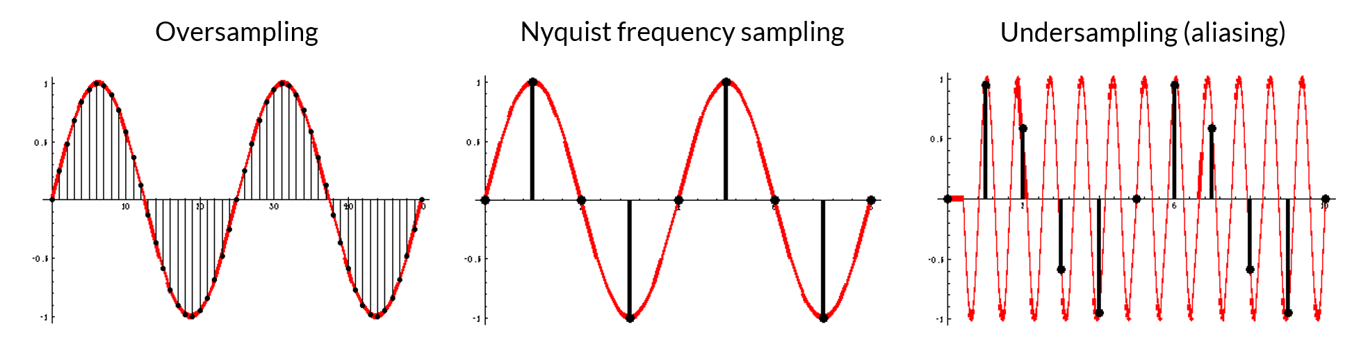
Digital sampling [information source]

Quantisation: Quantisation is the process of mapping the sampled values to a finite set of levels. This step is crucial because it converts the continuous range of amplitudes into discrete levels that can be represented digitally. Quantisation introduces a small error known as quantisation error, which is the difference between the actual sampled value and the quantised value. This error occurs because the continuous signal’s amplitude can take any value within a range, but the digital representation can only take on specific, predefined levels.

For example, imagine you are measuring have a continuous vibration, you get a series of amplitude values at regular intervals. However, these sampled values might not exactly match the discrete levels available in your digital system. Quantisation rounds these sampled values to the nearest available level. If your signal at a certain time is 3.13734 m/s and your measurement device is accurate to 0.1 m/s it will read 3.1 m/s, introducing a small error but making the signal convenient for digital processing.

Fourier Transform

The Fourier Transform is a mathematical technique that converts a time-domain signal into its frequency-domain representation, indicating how much of the signal’s quantity is distributed across different frequencies. This helps in understanding the spectral content of the signal, identifying features or the absence of features, such as harmonic components, which aid in describing and characterising the signal.

The formula of the Fourier transform is the following:

\[X(\omega) = \int_{-\infty}^{\infty} x(t) \cdot e^{-i \omega t} \, dt\]

\[\Downarrow\]

\[\text{where } \omega = 2\pi f\]

\[X(f) = \int_{-\infty}^{\infty} x(t) \cdot e^{-i 2\pi f t} \, dt\]

\[\Downarrow\]

\[\text{where } e^{-i \omega t} = \cos(\omega t) - i \sin(\omega t)\]

\[X(f) = \int_{-\infty}^{\infty} x(t) \cdot \left( \cos(2\pi f t) - i \sin(2\pi f t) \right) \, dt\]

The Fourier Transform works by projecting the time-domain signal (\(x(t)\)) onto a set of complex exponential functions (\(e^{-iωt}\)), each representing a different frequency. By multiplying the \(x(t)\) and \(e^{-iωt}\) and integrating, we measure how much each frequency component contributes to the signal. If \(x(t)\) and \(e^{-iωt}\) are aligned at a particular frequency, the integral yields a significant value, indicating the presence of that frequency in the signal, if they are not aligned, the positive and negative parts of the product cancel out, resulting in a smaller integral value.

Considering the complex components, we arrive to that Fourier Transform works by expressing a time-domain signal as a sum of sinusoidal functions, each with a specific frequency, amplitude, and phase. This allows for a detailed analysis of the signal’s frequency content.

Discrete Fourier Transform (DFT)

This package deals with digital signals which means they are composed of discreet values; therefore, a discreet version of the Fourier transform is needed. The Discrete Fourier Transform (DFT) is a mathematical technique used to convert a finite sequence of equally spaced samples of a function (signal) into a sequence of coefficients of a finite combination of complex sinusoids, ordered by their frequencies. The DFT of a sequence (\(x(n)\)) of length (\(N\)) is given by:

\[X_k = \sum_{n=0}^{N-1} x_n \cdot e^{-i 2\pi (\frac{k n}{N})},\]

where (\(k, n = 0, 1, 2, \ldots, N-1\))

Fast Fourier Transform (FFT)

The Fast Fourier Transform (FFT) is an efficient algorithm to compute the DFT and its inverse. This algorithm is highly efficient due to its divide-and-conquer approach, which reduces the computational complexity from (\(O(N^2)\)) to (\(O(N\log N)\)), and its use of symmetry and periodicity properties to minimise redundant calculations. The FFT is significant because it speeds up the computation of the DFT, making it feasible to process large datasets and real-time signals.

This is the algorithm used on the functions fft_from_time_domain_data() and rfft_from_time_domain_data() which are the core in the methods convert_to_frequency_domain() and convert_collection_to_frequency_domain() for TimeDomainData and for TimeDomainCollection objects respectively.

Inverse Fourier Transform (IFT)

The Inverse Fourier Transform (IFT) converts a frequency-domain representation back into the time-domain signal. The inverse DFT is given by:

\[g(t) = \int_{-\infty}^{\infty} G(\omega) \cdot e^{i 2\pi f t} \, df\]

\[x_n = \sum_{k=0}^{N-1} X_k \cdot e^{i 2\pi (\frac{k n}{N})}\]

where (\(k, n = 0, 1, 2, \ldots, N-1\))

This transformation is used in signal reconstruction to recreate the original time-domain signal from its frequency-domain representation. As well as for filtering, signal boosting or synthesis certain frequencies so when converted back to the time domain, resulting in a modified version of the original time signal.

Similarly to DFT to FFT there is Inverse Fast Fourier Transform (IFFT) algorithm. This is the algorithm used on the function time_domain_data_from_frequency_domain() by the means of the SciPy library. This function is the core in the methods convert_to_time_domain_data() and convert_collection_to_time_domain() for FrequencyDomainData and FrequencyDomainCollection objects respectively.

Signal (un)suitability for FFT

The Fast Fourier Transform (FFT) is a powerful tool, but there are certain conditions where a signal might not be suitable for FFT analysis [source]:

1. Uneven Time Step Size:

   • Issue: When the time intervals between successive samples of a signal are not uniform.

   • Impact: The FFT algorithm uses the Discrete Fourier Transform (DFT), which assumes a uniform grid of time points. Uneven sampling breaks this grid, leading to mathematical inconsistencies in the DFT computation.

   • Mitigation technic: if the signal has over sampling for the frequency content expected, interpolation can be performed to resample the signal at uniform intervals before applying the FFT (not yet implemented in the package).

2. Aliasing:

   • Issue: If the signal contains frequencies higher than half the sampling rate (Nyquist frequency), these frequencies will be aliased, appearing as lower frequencies in the FFT.

   • Impact: This can distort the frequency spectrum and lead to incorrect interpretations.

   • Mitigation technic: Ensuring the sampling rate is sufficiently high to capture all relevant frequency components.

3. Insufficient Sampling Rate:

   • Issue: If the sampling rate is too low, it may not capture the signal’s high-frequency components accurately.

   • Impact: This can result in a loss of information and an inaccurate frequency representation.

   • Mitigation technic: Ensuring the sampling rate is sufficiently high to capture all relevant frequency components.

4. Limited Resolution:

   • Issue: When a signal is too short, it may not contain enough information to accurately represent its frequency components.

   • Impact: The limited length of the signal can lead to poor frequency resolution in the Fourier Transform, making it difficult to distinguish between closely spaced frequency components. This can result in a blurred or smeared frequency spectrum.

   • Mitigation technic: By adding zeros (Zero Padding) to the end of the short signal, you can artificially increase its length. This does not add new information but improves the frequency resolution of the FFT by providing a finer grid in the frequency domain.

5. Discontinuities in the signal:

   • Issue: Abrupt change or discontinuity at the junction introduces high-frequency components that spread energy across multiple frequency bins in the Fourier Transform. If this discontinuity is real, we do want to describe it with high frequencies (impact loads) but sometimes these discontinuities are artificial.

   • Impact: This mismatch also leads to discontinuities and spectral leakage, where energy from one frequency bin spreads into others, distorting the frequency representation.

   • Examples: Signals with different start and end, when stitching signal together, non-periodic signals.

   • Mitigation technic: Applying a window function (Windowing) to the signal before performing FFT can reduce spectral leakage by tapering the signal at the boundaries.

6. Non-Stationary Signals:

   • Issue: FFT assumes that the signal’s statistical properties do not change over time (stationarity).

   • Impact: For non-stationary signals, where properties like mean and variance change over time, the FFT may not provide a meaningful frequency representation.

   • Examples: Measurements of stress and strain in materials over time can show non-stationary behavior due to varying loads, structural nonlinearities and changing environmental conditions.

   • Mitigation technic: Make sure the segment of time domain data that will be analysed does not have a wide range of varying loads, structural nonlinearities or changing environmental conditions. Short-Time Fourier Transform (STFT): Dividing the signal into smaller segments and applying the Fourier Transform to each segment, and then combines the results to provide a time-frequency representation of the signal (resolution is lost). (currently this can me done manually in the current tool but there are plans to automate this) Wavelet Transform: This method does not use the FT but it is similar, instead of the Euler equation uses wavelets, which are localised in both time and frequency. This allows to analyse signals that have time-varying frequency content, which is particularly useful for non-stationary signals. (To be implemented)

Note

Impact loads, short bursts, or transient events produce non-stationary signals. However, the FFT is still regularly used to analyse these signals. Despite some fundamental issues with applying the FFT to non-stationary signals, there are workarounds:

1. Keep in mind that due to discontinuities, there may be unexpected and artificial high-frequency content.

2. If possible, isolate different transient events to reduce discontinuities.

3. Consider that normalisation techniques for windowing and signal length are derived from stationary signals. Therefore, amplitude and power values in the frequency domain may not represent real-world values accurately. In such situations, investigating the total amount of energy can be more meaningful.

In the package there checks are performed for suitability in FFT. The function check_td_ft_suitability() runs check_time_stamps_intervals(), check_stationary() and check_periodicity(). These functions are also called by the methods convert_to_frequency_domain() and convert_collection_to_frequency_domain() for TimeDomainData and for TimeDomainCollection objects respectively. There are also other functions implemented to apply the mitigation techniques previously mentioned, these are explained in more detail in the next section Preparing Data for FFT.

Warning

These checks are performed in the Signal Processing Tool. When a check fails a warning is raised, but the process will continue. Consider improving the signal contents, or resampling to prevent possible mathematical inaccuracies in the tool.

Preparing Data for FFT

Before performing the FFT, it is essential to prepare the data properly to make sure that the signal is suitable for the FFT.

Windowing

Windowing involves applying a window function to a signal to reduce spectral leakage. Common window functions include Hamming, Hanning, Blackman, and Rectangular windows. The purpose of windowing is to minimise discontinuities at the boundaries of the sampled signal, which can cause artifacts in the frequency domain.

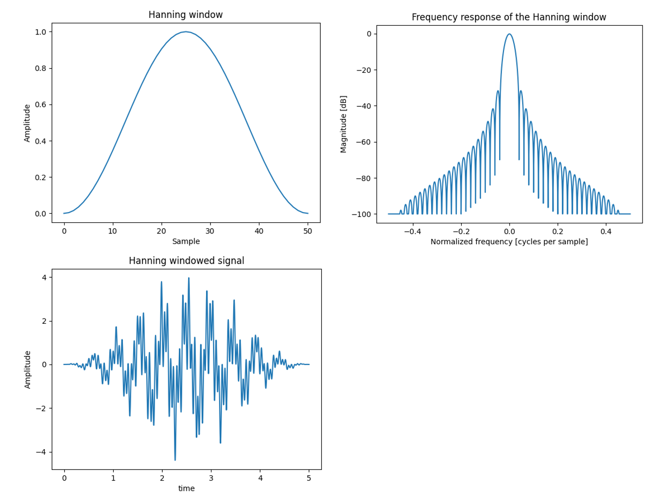
Since these windows alter the shape of the original signal it must be normalised so that the magnitude of the quantities is scaled correctly, maintaining the correct amplitude levels in the frequency domain, especially when comparing signals or performing further analysis. It is important that the normalisation factor is different per window type as well as if the results of the FFT is used to calculate the amplitudes or the energy content.

The types of windows and window normalisation factors used in this tool apply_window are the following:

Window Type	Normalisation for Amplitude	Normalisation for Energy
Rectangular	1.00	1.00
Hanning	2.00	1.63
Hamming	1.85	1.59
Blackman	2.38	1.73
Bartlett	2.00	1.33

This is the procedure used by the function apply_window which is an important step in the methods convert_to_frequency_domain() and convert_collection_to_frequency_domain() for TimeDomainData and for TimeDomainCollection objects respectively.

Zero-Padding

Zero-padding involves adding zeros to the end of the signal to increase its length before performing the FFT. This increases the frequency resolution of the FFT output without changing the actual content of the signal, helping to better identify and distinguish closely spaced frequency components.

In the Signal Processing tool zero padding is done with the function zero_pad_time_domain_data() which is used in the methods zero_pad_time_domain() for the TimeDomainData Class.

Eliminating noise

Is not needed to run the FFT but can clean up the results so that you only have the meaningful data.

Note

To be implemented.

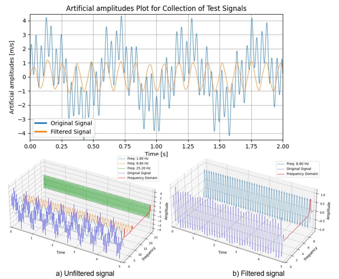
Filtering

Filters are used in signal processing to enhance the quality and clarity of the data. In structural engineering, they are used for isolating specific frequency components, removing noise, and focusing on relevant signal features. This allows to accurately describe forces as well as structural properties and potential issues. By applying filters, the data becomes more reliable and easier to interpret, leading to better-informed maintenance decisions and ensuring the safety and longevity of structures.

Filtering in signal processing involves manipulating a signal to enhance desired components and suppress unwanted ones. This is achieved using various types of filters, such as low-pass, high-pass, band-pass, and band-stop filters. Each filter type targets specific frequency ranges: low-pass filters allow frequencies below a certain cutoff to pass through, high-pass filters allow frequencies above a certain cutoff, band-pass filters allow a specific range of frequencies, and band-stop filters block a specific range. By applying these filters, it can clean up signals, remove noise, and focus on the relevant data, making it easier to analyse and interpret the information accurately.

Common implementations of filters include Butterworth, Chebyshev, and Elliptic filter designs, each with different characteristics in terms of passband ripple and roll-off rate. This Signal Processing Tool has the apply_filter_to_signal() function which is used in several methods of TimeDomainData and TimeDomainCollection objects. This function uses the uses SciPy library butter function which uses a the Butterworth to filter digital and analogy signals. This function only has high, low and band-pas filters but not band-stop filter.

Manipulations performed after the FFT

Even after preparing the time domain signal for FFT some manipulations of the FFT results are needed to obtain data with accurate and useful magnitudes of the Frequency Domain quantities.

Length Normalisation

Length normalisation ensures that the amplitudes of the frequency components are correctly scaled by dividing the FFT results by the number of data points, providing consistent amplitude values regardless of the signal length. This normalisation is crucial for accurate interpretation and comparison of frequency domain data, especially when analysing signals of varying lengths. When the signal is stationary, this process provides accurate values for the magnitudes of quantities like amplitude and power, making the analysis reliable and meaningful.

In the Signal Processing Tool length normalisation is done automatically in the function amplitude_spectrum_from_time_domain_data() which is used in the methods convert_to_time_domain_data() and convert_collection_to_time_domain_data() for TimeDomainData and FrequencyDomainCollection objects.

Length normalisation assumes the signal is stationary, so the quantities arrived form the FT can be average out in the signals time. For this reason, length normalisation is not always recommended for non-stationary signals, such as those involving impact loads, short bursts, transient events, or time-varying structural properties. In these cases, the signal characteristics change over time, and normalising by the number of data points can distort the true amplitude and power of the frequency components. In such scenarios, other techniques such as Short-Time Fourier Transform or Wavelet transform allow for the analysis of signals with time-varying frequency content.

Similarly, if the signal has been zero-padded (forcing it to be non-stationary), length normalisation can lead to incorrect scaling, as the added zeros artificially increase the signal length without contributing to the actual signal content. In this case, if the original time signal data length is known, it can be used for normalisation (the tool does not have this functionality it will use the length of the signal even if its zero-padded).

Therefore, consideration is needed to determine whether length normalisation is appropriate based on the specific nature of the signal being analysed, since the magnitudes of the quantities in the frequency domain might be distorted. However, in many cases, the exact magnitudes of the quantities are not necessary; the information about what frequency the peaks appear or the relative magnitude between the frequency components is often sufficient.

Amplitudes and Phase Angles

When performing a FT on a time-domain signal, the result is a set of complex numbers that represent both the amplitude and phase of the frequency components.

The amplitude of each frequency component indicates the strength or magnitude of that frequency in the signal. To obtain the amplitude, you need to take the absolute value (or magnitude) of the complex FFT result.

The phase angle represents the shift of each frequency component relative to the start of the time-domain signal. To calculate the phase angle, you use the 2nd arctangent function. The phase angle provides information about the timing of the frequency components, which is essential for reconstructing the original signal or understanding its behaviour.

In this tool it is implemented using NumPy library in convert_fft_to_real_positive_sided_spectrum which is

used in the methods convert_to_frequency_domain() and convert_collection_to_frequency_domain() for TimeDomainData and TimeDomainCollection objects respectively. Inversely when going form frequency domain to time domain the tool uses the function reconstruct_2sided_complex_spectrum() which is indirectly used in which is used in the methods convert_to_time_domain() and convert_collection_to_time_domain() for FrequencyDomainData and FrequencyDomainCollection objects respectively.

Two-Sided and Single-Sided Spectrum

The result of the Fourier Transform provides a Two-Sided Spectrum, which includes both positive and negative frequency components. This is because the FT of a real-valued time-domain signal is inherently complex. The negative frequencies are the complex conjugates of the positive frequencies. If the time signal is real-valued (like in all structural engineering cases), the frequency domain is symmetrical, and the negative frequencies mirror the positive side. This mirroring is sometimes represented around the DC component (0th frequency), which better depicts the notion of negative frequencies, but often it is mirrored around the Nyquist frequency (max frequency) because the FFT is periodic, and the Nyquist frequency represents the highest frequency that can be accurately represented from the time sampling size. This periodicity causes the spectrum to wrap around at the Nyquist frequency, effectively mirroring the positive frequencies into the negative frequency range.

So, for real-valued time signals the negative redundant content is redundant, nevertheless these components do contain part of the energy of the signal so if we are interested that the quantities in the frequency domain are accurate, we have to take them into account. Follow these steps to convert a Two-Sided Spectrum to a Single-Sided Spectrum:

• Keep the Positive Frequencies: Keep only the positive frequency components from the Two-Sided Spectrum.

• Double the Amplitudes: Multiply the amplitudes of the positive frequencies by two to account for the energy that was originally split between the positive and negative frequencies. However, do not double the amplitude at the zero frequency (DC component) and the Nyquist frequency (if it exists), as these are unique and do not have corresponding negative frequencies.

As mentioned before, this conversion can be done when the original signal is real-valued, and the analysis focuses on the magnitude of the frequency components. It is not applicable for complex-valued signals, as they do not exhibit the ame symmetry properties.

This tool uses the SciPy library to perform the FFT and it outputs the data mirrored around the Nyquist frequency. Afterwards the function convert_double_sided_to_real_single_sided_spectrum() is used which is indirectly used in the methods convert_to_frequency_domain() and convert_collection_to_frequency_domain() for TimeDomainData and TimeDomainCollection objects respectively. Inversely when going form frequency domain to time domain the tool uses the function reconstruct_2sided_complex_spectrum() which is indirectly used in the methods convert_to_time_domain() and convert_collection_to_time_domain() for FrequencyDomainData and FrequencyDomainCollection objects respectively.

Error

Documentation to be extended on this topic.

Procedure to calculate to RMS values

The procedure to calculate the Root Mean Square (RMS) values from a time-domain signal involves several steps:

1. Apply filter to the entire signal to remove low frequency content or other unwanted signals.

2. Segment signal if averaging is required. Define segments:

   1. Overlap typical optimal 50-60% (typically choose 50%)

      b) Segment length (N) can be defined by duration of segment (1s, 0.25s) or more rigorously by balancing bias and random error.

      • Defined segment length:

        \[N = \frac{T_{\text{segment}}}{\Delta t}\]
        \[M = \frac{T_{\text{tot}}}{(1 - \text{OL}) \cdot T_{\text{segment}}}\]

      • Balancing error: look for a combination of highest N and M that produce the highest relative difference between max and mean value of next step.

      • Preferably to choose N in a power of 2.

   3. Segment length (N) determines frequency resolution

3. Calculate double sided linear spectrum (Amplitude spectrum) of the windowed segment, including amplitude correction factor for windowing and signal length:

   \[X_w(m, k) = \frac{A_w}{N} \sum_{n=0}^{N-1} \left( x_{m,n} \cdot w_n \right) e^{-i 2\pi \frac{k n}{N}}\]

4. Convert so single sided Amplitude spectrum. Only use positive values, Double values except DC (k=0), get rid of

negative side of the spectrum.

\[\begin{split}X_{+w}(m, k) = \begin{cases} 2 \cdot X_w(m, k) & \text{if } k \ne 0 \\ X_w(m, k) & \text{if } k = 0 \end{cases}\end{split}\]

In the package length normalisation (dividing FFT by N) is done after converting to single sided spectrum to provide the option of skipping the length normalisation. Order does not change the outcome.

5. Calculate the Power Spectral Density function (PSD) (\(G_{xx}(m, k)\) in books notation)

   \[\text{PSD}_{(m, k)} = \frac{1}{\Delta f \cdot N \cdot \text{ENBW}} \left| X_w(m, k) \right|^2\]

   Note

   Be sure to use the double sided spectrum.

6. If segmenting was performed, average the values

\[\text{PSD}_{\text{ave}}(k) = \frac{1}{M} \sum_{m=1}^{M} \text{PSD}_{(m, k)}\]

7. Calculate RMS form PSD

\[x_{\text{RMS}}(k_1, k_2) = \sqrt{ \Delta f \cdot \sum_{k = k_1}^{k_2} \text{PSD}_{\text{ave}}(k) }\]

Spectral Analysis for Vibration Signals

1. Peak Values and Peak-to-peak

   • Definition: Peak values represent the maximum amplitude observed in a vibration signal. They are crucial for identifying extreme events and potential faults in machinery.

   • Significance: High peak values can indicate severe mechanical issues such as impacts, misalignment, or bearing failures. Monitoring peak values helps in early fault detection and preventive maintenance.

2. Root Mean Square (RMS) Values for Signal Strength

   • Definition: RMS value is a statistical measure of the magnitude of a varying signal. It provides an indication of the overall energy or power of the vibration signal.

   • Calculation: The RMS value is calculated as:

     \[x_{\text{RMS}} = \frac{1}{N} \sum_{n=0}^{N-1} x(n)^2\]

     where (\(x(n)\)) is the signal amplitude and (N) is the number of samples.

   • Significance: RMS values are used to assess the overall vibration level and compare it against acceptable thresholds. High RMS values can indicate excessive vibration and potential damage to machinery.

3. Octaves

4. Resonance and Its Identification

   • Definition: Resonance occurs when the frequency of an external force matches the natural frequency of a system, causing large amplitude oscillations.

   • Identification: Resonance can be identified by analyzing the frequency spectrum of the vibration signal. Peaks at specific frequencies indicate resonance.

   • Significance: Identifying resonance is crucial for preventing excessive vibrations that can lead to structural damage or failure.

5. Amplification Factor and Its Implications

   • Definition: The amplification factor is the ratio of the output amplitude to the input amplitude at a specific frequency. It indicates how much the vibration is amplified at resonance.

   • Significance: High amplification factors at resonance frequencies can lead to significant mechanical stress and potential failure. Understanding amplification factors helps in designing systems to avoid resonant conditions.

6. Damping and Its Effects on Signal Behavior

   • Definition: Damping is the process by which energy is dissipated in a vibrating system, reducing the amplitude of oscillations over time.

   • Types of Damping: Common types include viscous damping, Coulomb damping, and structural damping.

   • Effects: Damping affects the amplitude and decay rate of vibrations. Adequate damping is essential for controlling vibrations and preventing resonance.

   • Significance: Analysing damping characteristics helps in designing systems with appropriate damping to ensure stability and longevity.

Wavelet Transform

Note

These notes have not been implemented in the tool yet.

1. Introduction to Wavelet Transform and Its Advantages over Fourier Transform

   • Definition: The wavelet transform is a mathematical technique that decomposes a signal into components at various scales or resolutions. Unlike the Fourier transform, which uses sinusoidal basis functions, the wavelet transform uses wavelets—functions that are localised in both time and frequency.

   • Advantages over Fourier Transform:

     • Time-Frequency Localisation: Wavelets provide better localization in both time and frequency domains, making them suitable for analysing non-stationary signals where frequency components change over time.

     • Multi-Resolution Analysis: Wavelet transform allows for multi-resolution analysis, enabling the examination of signal details at different scales.

     • Adaptability: Wavelets can be adapted to different types of signals, providing more flexibility in signal analysis.

     • Noise Reduction: Wavelet transform is effective in denoising signals, as it can separate noise from the signal more efficiently than the Fourier transform.

2. Applications of Wavelet Transform in Signal Analysis

   • Vibration Analysis: Identifying transient events and faults in machinery by analyzing vibration signals at different scales.

   • Biomedical Signal Processing: Analysing ECG and EEG signals to detect abnormalities and diagnose medical conditions.

   • Image Processing: Enhancing and compressing images by decomposing them into wavelet coefficients.

   • Audio Processing: Denoising and compressing audio signals while preserving important features.

   • Geophysics: Analysing seismic signals to detect and characterize geological structures.

Frequency domain dynamic response

From input and transfer function, multiply in the frequency domain to arrive to response and than transfer back to time domain.

SBR Trillingsrichtlijnen

SBR stands for Stichting BouwResearch (Foundation for Building Research). It is known for publishing guidelines related to vibration measurements and assessments in buildings. These guidelines are widely used in engineering, construction, and environmental impact studies.

SBR Guidelines Overview

There are three main SBR guidelines, each addressing a different aspect of vibration:

• SBR-A – Damage to buildings: Focuses on assessing whether vibrations (e.g. from construction or traffic) can cause structural damage to buildings.

• SBR-B – Nuisance for people in buildings: Evaluates whether vibrations cause discomfort or annoyance to occupants. It considers building function, vibration source, and whether the situation is existing, modified, or new. Assessment is based on threshold values A1, A2, and A3 for vibration intensity.

• SBR-C – Impact on vibration-sensitive equipment: Used when vibrations might interfere with sensitive instruments or processes (e.g. in laboratories or hospitals).

These guidelines are not part of Dutch law but are considered industry standards and are often referenced in contracts, environmental assessments, and legal disputes. They are especially relevant in areas like Groningen, where induced earthquakes from gas extraction have raised concerns about vibration-related damage and nuisance.

You can find these documents in the Knowledge Library of AT&R - Vibration Engineering.

Vibration Measurements – Nuisance – SBR Guideline B

Measurement and assessment guideline B, “Nuisance for people in buildings”, provides standards for measuring and evaluating vibration nuisance experienced by individuals. The guideline distinguishes between the function of the building, the type of vibration source, and whether the situation is existing, modified, or new.

The assessment in the guideline is based on three threshold values: \(A_{\text{1}}\), \(A_{\text{2}}\), and \(A_{\text{3}}\):

1. \(A_{\text{1}}\) is the lower target value for vibration intensity \(V_{\text{max}}\).

2. \(A_{\text{2}}\) is the upper target value for vibration intensity \(V_{\text{max}}\).

3. \(A_{\text{3}}\) is the target value for the vibration intensity \(V_{\text{per}}\) (average over time).

In general, the relationship between these values is \(A_{\text{3}}\) < \(A_{\text{1}}\) < \(A_{\text{2}}\) Compliance with the target values is achieved if:

• The maximum vibration intensity in a room (\(V_{\text{max}}\)) is less than \(A_{\text{1}}\), or;

• The maximum vibration intensity (\(V_{\text{max}}\)) is less than A2, and the average vibration intensity over the assessment period (\(V_{\text{per}}\)) is less than A3.

The target values in the guideline are based, among other things, on the function of the building where the vibrations are assessed and the nature of the vibration source.

Determination of Vibration Strength

The vibration strength in buildings is assessed through a multi-step signal processing method applied to measured vibration data. The procedure includes weighting, effective value calculation, statistical processing, and comparison with target values.

Note

This method applies to each measurement point and direction individually.

Steps:

1. Weighting of the vibration signal (\(v(t)\)):

   Apply a frequency-dependent weighting function to the measured acceleration or velocity signal. For velocity signals use:

   \[\left| H_v(f) \right| = \frac{1}{v_0} \cdot \frac{1}{\sqrt{1 + \left( \frac{f_0}{f} \right)^2 }}\]

2. Progressive effective value (\(V_{\text{eff}}(t)\)):

   Compute the moving RMS value using an exponential time window (integration time: \(\tau=0.125s\)).

   \[ \begin{align}\begin{aligned}V_{\text{eff}}(t) = \sqrt{ \frac{1}{\tau} \int_0^t g(\xi) v^2(t - \xi) d\xi }\\\quad g(\xi) = \exp(-\xi / t)\end{aligned}\end{align} \]

3. Maximum effective value per 30-second interval (\(V_{\text{eff,max,30,i}}\)):

   Determine the peak value of \(V_{\text{eff}}(t)\) in each 30-second interval. Exclude disturbances if justified.

4. Maximum effective value over the entire measurement (\(V_{\text{eff,max}}\)):

   Identify the highest \(V_{\text{eff}}(t)\) across the full measurement duration.

5. Statistical processing (optional):

   Apply log-normal distribution to the top 15 values of \(V_{\text{eff,max,30,i}}\). Compute \(V_{\text{eff,max,stat}}\) using mean and standard deviation with a safety factor (β).

6. Maximum vibration strength (\(V_{\text{max}}\)):

   Defined as the highest value of \(V_{\text{eff,max}}\) or \(V_{\text{eff,max,stat}}\). Evaluated per assessment period (day, evening, night).

7. Vibration strength over the assessment period (\(V_{\text{per}}\)):

   Compute the RMS of \(V_{\text{eff,max,30,i}}\) over the measurement period. Adjust for the ratio of source activity time (\(T_b\)) to total assessment time (\(T_o\)).

Assessment:

• Compare \(V_{\text{max}}\) and \(V_{\text{per}}\) against target values A1, A2, and A3.

• Compliance is achieved if: - \(V_{\text{max}} < A1\), or - \(V_{\text{max}} < A2\) and \(V_{\text{per}} < A3\).