Creating signals

Three options are available for the user to create signals in the time domain:

Manual creation of a signal: The user provides the time and the amplitude values as lists.
Import signal from a file: The signal is imported from a (Sigicom) csv-file or xlsx-file.
Use built-in signal generators: Create a signal with sinusoidal amplitudes, Heaviside, Kronecker, Dirac or Ricker-Wavelet methods.

In this section these methods are explained in more detail.

Time Domain Data

In this tool, the signal is referred to as the raw time-domain data. It consists of two lists: one containing time values and the other containing corresponding amplitude values. Additional metadata related to the signal is stored in a TimeDomainData object, which encapsulates information such as name, units, sampling rate, duration, and other relevant attributes.

The time domain data can be added to a collection of multiple signals, which is managed by the TimeDomainCollection class. This class provides the functionality to manage multiple time-domain signals, and execute functions on all contained signals. The collection is added to the project instance.

Manual creation of a signal

Any signal can be provided manually by specifying the time and amplitude values as lists. The lists should be of equal length. For this the function create_time_domain_data() is used.

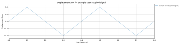
The following example creates a signal with 9 samples, with amplitudes varying between -1 and 1, at specified time stamps.

time_domain_data = project.create_time_domain_data(
    name='Example User Supplied Signal',
    amplitudes=[0, 1, 0, -1, 0, 1, 0, -1, 0],
    time_stamps=[0, 0.1, 0.2, 0.3, 0.4, 0.5, 0.6, 0.7, 0.8],
    collection_name='Example Collection',
    amplitude_type='displacement',
    amplitude_units='mm',
    time_stamps_units='seconds')

Import signal from a file

The Signal Processing Tool provides multiple options for importing signals from a file. Signals can be imported from a csv-file or xlsx-file. Also files from Sigicom can directly be imported. The file should contain two columns: one for the time values and one for the amplitude values. The first row should contain the header with the names of the columns.

The function create_time_domain_data_from_file() is used to import a signal from a file. The function requires the path to the file, the names of the columns containing the time and amplitude values, the units of the time and amplitude values and the type of signal.

time_domain_data = project.create_time_domain_data_from_file(
    name='Example Signal From File',
    file='path_to_your_file/file_name.xlsx',
    time_column: 'Timestamp',
    amplitude_column: 'Value',
    amplitude_type='acceleration',
    amplitude_units='mm/s^2',
    time_stamps_units='seconds')

You can also load signals from multiple csv- or xlsx-files in same collection. This is done with the function create_time_domain_collection_from_file().

For Sigicom files a dedicated function create_time_domain_data_from_sigicom_csv() is available

time_domain_data = project.create_time_domain_data_from_sigicom_csv(
    name='Example Sigicom Signal From File',
    file='path_to_your_file/file_name.csv',
    amplitude_type='acceleration',
    amplitude_units='mm/s^2',
    time_stamps_units='seconds')

You can also load multiple signals from Sigicom files. This is done with the function create_time_domain_collection_from_sigicom_csv().

Use built-in signal generators

The Signal Processing Tool includes several built-in signal generators that can be used to create common types of signals. These generators are described in this section.

Sinusoidal Function

The sinusoidal function create_sinusoidal_time_domain_data() models harmonic loads or vibrations at specific frequencies, making it a fundamental tool in structural dynamics and signal analysis. In vibration studies, it is particularly useful for simulating machinery-induced oscillations, analysing resonances, and evaluating a system’s frequency response and modal behaviour. Mathematically, the sinusoidal signal is defined by a continuous oscillation, typically expressed as:

\[A \cdot \sin(2\pi f t + \phi)\]

or as a sum of such terms in the multi-sinusoidal case. This flexibility makes it ideal for exploring how structures respond to periodic or quasi-periodic excitations over time.

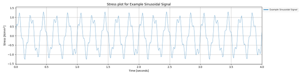
In this example we create a signal of 4 seconds for stresses. The signal consists of two harmonics: one with an amplitude of 1.0 N/mm2 and a frequency of 5 Hz, and another with an amplitude of 0.3 N/mm2 and a frequency of 18 Hz. The second harmonic has a phase shift of 45 degrees. The resulting signal is a combination of these two sinusoidal components.

time_domain_data = project.create_sinusoidal_time_domain_data(
    name='Example Sinusoidal Signal',
    harmonic_amplitudes=[1.0, 0.3],
    harmonic_frequencies=[5, 18.0],
    harmonic_phase_shift=[0.0, 45.0],
    duration=4,
    amplitude_type='stress',
    amplitude_units='N/mm2',
    time_stamps_units='seconds')

Dirac Delta Function (Impulse Response)

The Dirac delta function (use create_special_time_domain_data()) represents an idealised instantaneous force or shock, such as a hammer hit or impact load. The function can be used in structural and vibration analysis for studying how systems respond to sudden, high-intensity excitations.

In vibration analysis, the Dirac delta is used to evaluate the impulse response of a system — that is, how the structure behaves when subjected to a force that occurs over an infinitesimally short time. This is particularly useful in modal analysis, system identification, and dynamic testing.

Mathematically, the Dirac delta is not a function in the traditional sense but a distribution. It has infinite amplitude at a single point, is zero everywhere else, and integrates to unit area:

\[\int_{-\infty}^{\infty} \delta(t - t_0) \, dt = 1\]

In numerical simulations, it is typically approximated by a narrow pulse or a scaled discrete value to maintain its unit area property.

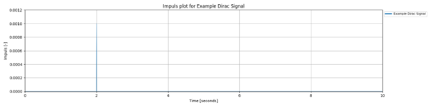
In the following example the event is set at time = 2.0 seconds. The functions calculates such that the total area under the signal is 1. This approximates the unit impulse behavior of the Dirac delta. Note that the amplitude is not an input and the default signal duration 10 seconds, and the default sampling rate is 100 Hz.

my_time_domain_data = project.create_special_time_domain_data(
    name='Example Dirac Signal',
    signal_type='dirac',
    event_time=2.0,
    amplitude_type='impuls',
    amplitude_units='-',
    time_stamps_units='seconds')

The peak amplitude of the Dirac delta signal is determined by the sampling rate and duration of the signal:

\[\text{Peak value} = \frac{1}{f_s \cdot T}\]

where \(\\T\) is the duration of the signal, and \(f_s\) is the sampling rate in Hz.

Heaviside Step Function

The Heaviside step function (use create_special_time_domain_data()) models the sudden application of a load that remains constant, such as a weight dropped and left on a beam. It is commonly used in structural and vibration analysis to simulate step loads — forces or displacements that turn on abruptly and persist over time.

In vibration studies, the Heaviside function is essential for analysing the step response of a system: how a structure reacts when subjected to a load that is suddenly applied and maintained. This helps engineers understand transient behaviour, damping characteristics, and long-term stability.

\[\begin{split}H(t - t_0) = \begin{cases} 0, & t < t_0 \\ 1, & t \geq t_0 \end{cases}\end{split}\]

Where \(t0t_0t0\) is the time at which the load is applied. The function jumps from 0 to 1 at \(t0t_0t0\), representing the onset of the constant load.

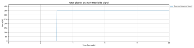
In the following example the event is set at time = 3.0 seconds, with an amplitude of 350 N. The default duration of 10 seconds is applied and the sampling rate is 100 Hz.

time_domain_data = project.create_special_time_domain_data(
    name='Example Heaviside Signal',
    signal_type='heaviside',
    event_time=3.0,
    amplitude=350.0,
    amplitude_type='force',
    amplitude_units='N',
    time_stamps_units='seconds')

Kronecker Delta Function

The Kronecker delta function (use create_special_time_domain_data()) is used in discrete systems, especially in numerical simulations and finite element models, where signals or forces are applied at specific time steps or nodes. It is ideal for modeling node-specific excitations or discrete-time events in vibration and structural analysis.

In vibration studies, the Kronecker delta is useful when working with discrete-time systems, such as time-stepped simulations or matrix-based formulations. It allows you to apply a force or condition at a specific index in time or space, making it a precise tool for localised excitation.

Mathematically, the Kronecker delta is defined as:

\[\begin{split}\delta_{ij} = \begin{cases} 1, & i = j \\ 0, & i \ne j \end{cases}\end{split}\]

It evaluates to 1 when the indices match and 0 otherwise, making it a simple yet powerful tool for indexing and selection in discrete models.

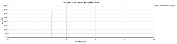
In the following example the event is set at time = 3.0 seconds, with an amplitude of 350 N. The default duration of 10 seconds and sampling rate of 100 Hz are applied.

time_domain_data = project.create_special_time_domain_data(
   name='Example Kronecker Signal',
   signal_type='kronecker',
   event_time=3.0,
   amplitude=350.0,
   amplitude_type='force',
   amplitude_units='N',
   time_stamps_units='seconds')

Ricker Wavelet (Mexican Hat Wavelet)

The Ricker wavelet function, also known as the Mexican hat wavelet, create_ricker_wavelet_time_domain_data() is commonly used to simulate transient dynamic loads, such as seismic events or short-duration forces. It is particularly valuable in structural and vibration analysis for studying transient responses and wave propagation through materials and structures.

In vibration studies, the Ricker wavelet helps capture the localized nature of dynamic events — combining both time and frequency information. This makes it ideal for analyzing how structures respond to short, oscillatory bursts of energy, such as those caused by earthquakes or traffic-induced shocks.

Mathematically, the Ricker wavelet is an oscillatory function with a central peak and decaying oscillations on either side. It is defined as the second derivative of a Gaussian function:

\[\psi(t) = \left(1 - 2\pi^2 f^2 t^2\right) e^{-\pi^2 f^2 t^2}\]

Where: \(f\) is the central frequency of the wavelet, \(t\) is time.

This formulation produces a symmetric wavelet with a sharp peak and diminishing side lobes, ideal for modeling localised energy bursts.

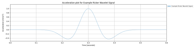
The following example creates a Ricker wavelet signal with a center frequency of 5 Hz, a duration of 0.6 seconds.

time_domain_data = project.create_ricker_wavelet_time_domain_data(
    name='Example Ricker Wavelet Signal',
    center_frequency=5.0,
    centered=False,
    duration=0.6,
    sampling_rate=200,
    collection_name='S1',
    amplitude_type='acceleration',
    amplitude_units='mm/s^2',
    time_stamps_units='seconds')